Basics
First, we import everything from Dionysus:
>>> from __future__ import print_function   # if you are using Python 2
>>> import dionysus as d
Simplices
A simplex is simply a list of vertices. It’s represented by the Simplex class:
>>> s = d.Simplex([0,1,2])
>>> print("Dimension:", s.dimension())
Dimension: 2
We can iterate over the vertices of the simplex.
>>> for v in s:
...     print(v)
0
1
2
Or over the boundary:
>>> for sb in s.boundary():
...     print(sb)
<1,2> 0
<0,2> 0
<0,1> 0
Simplices can store optional data, and the 0 reported after each boundary edge is the default value of the data:
>>> s.data = 5
>>> print(s)
<0,1,2> 5
We can use closure() to generate all faces of a set of
simplices. For example, an 8-sphere is the 8-dimensional skeleton of the
closure of the 9-simplex.
>>> simplex9 = d.Simplex([0,1,2,3,4,5,6,7,8,9])
>>> sphere8  = d.closure([simplex9], 8)
>>> print(len(sphere8))
1022
Filtration
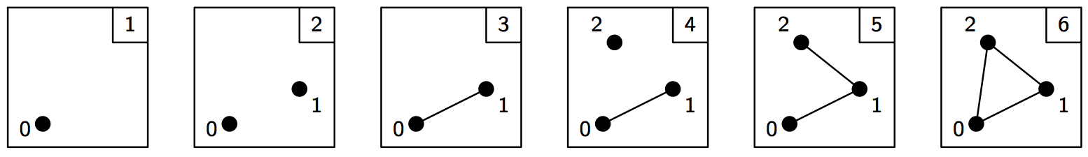
A filtration is a nested sequence of simplicial complexes, \(K_1 \subseteq K_2 \subseteq \ldots \subseteq K_n\). Without loss of generality, we can assume that two consecutive complexes in the filtration differ by a single simplex, so we can think of a filtration as a sequence of simplices.
In Dionysus, a filtration is represented by a special class,
Filtration, that supports both iterating over the
simplices and looking up an index given a simplex. A filtration can be
sort()ed. By default this orders
simplices by their data, breaking ties by dimension, and then
lexicographically.
>>> simplices = [([2], 4), ([1,2], 5), ([0,2], 6),
...              ([0], 1),   ([1], 2), ([0,1], 3)]
>>> f = d.Filtration()
>>> for vertices, time in simplices:
...     f.append(d.Simplex(vertices, time))
>>> f.sort()
>>> for s in f:
...    print(s)
<0> 1
<1> 2
<0,1> 3
<2> 4
<1,2> 5
<0,2> 6
We can lookup the index of a given simplex. (Indexing starts from 0.)
>>> print(f.index(d.Simplex([1,2])))
4
Persistent Homology
Applying homology functor to the filtration, we get a sequence of homology groups, connected by linear maps:
\(H_*(K_1) \to H_*(K_2) \to \ldots \to H_*(K_n)\). To compute decomposition of this sequence, i.e., persistence barcode,
we use homology_persistence(), which returns its internal representation of the reduced boundary matrix:
 >>> m = d.homology_persistence(f)
 >>> for i,c in enumerate(m):
 ...     print(i, c)
 0
 1
 2 1*0 + 1*1
 3
 4 1*1 + 1*3
 5
We can manually extract the persistence pairing from the reduced matrix:
>>> for i in range(len(m)):
...     if m.pair(i) < i: continue      # skip negative simplices
...     dim = f[i].dimension()
...     if m.pair(i) != m.unpaired:
...         print(dim, i, m.pair(i))
...     else:
...         print(dim, i)
0 0
0 1 2
0 3 4
1 5
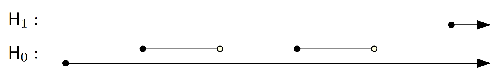
But we can also use the init_diagrams() function, by providing it access to the filtration:
>>> dgms = d.init_diagrams(m, f)
>>> print(dgms)
[Diagram with 3 points, Diagram with 1 points]
>>> for i, dgm in enumerate(dgms):
...     for pt in dgm:
...         print(i, pt.birth, pt.death)
0 1.0 inf
0 2.0 3.0
0 4.0 5.0
1 6.0 inf
Notice that init_diagrams() uses the data stored in
the simplices, instead of the index pairing we printed out in the previous
example.
homology_persistence() knows several methods of
persistence computation. These can be specified with the method keyword
argument:
>>> m = d.homology_persistence(f, method = 'column')
Homology. Dionysus doesn’t compute homology directly, but we can get it as a by-product of persistent homology.
>>> f = d.Filtration(sphere8)
>>> f.sort()
>>> m = d.homology_persistence(f, prime=2)
>>> dgms = d.init_diagrams(m, f)
>>> for i, dgm in enumerate(dgms):
...     print("Dimension:", i)
...     for p in dgm:
...         print(p)
Dimension: 0
(0,inf)
Dimension: 1
Dimension: 2
Dimension: 3
Dimension: 4
Dimension: 5
Dimension: 6
Dimension: 7
Dimension: 8
(0,inf)
Relative persistent homology
It’s possible to compute persistent homology of a filtration relative to a subcomplex:
\(H_*(K_1, L_1) \to H_*(K_2, L_2) \to \ldots \to H_*(K_n, L_n)\), where \(L_i = K_i \cap L_n\).
To accomplish this,
homology_persistence() takes an extra argument,
relative, to specify the subcomplex, \(L_n\). This subcomplex is
represented by a Filtration, but the ordering of
the simplices in it doesn’t matter, only their presence.
For example, homology of a triangle relative to its boundary has a single class in dimension 2:
>>> f = d.Filtration(d.closure([d.Simplex([0,1,2])], 2))
>>> f.sort()
>>> f1 = d.Filtration([s for s in f if s.dimension() <= 1])

>>> m = d.homology_persistence(f, relative = f1)
>>> dgms = d.init_diagrams(m, f)
>>> for i, dgm in enumerate(dgms):
...     print("Dimension:", i)
...     for p in dgm:
...         print(p)
Dimension: 0
Dimension: 1
Dimension: 2
(0,inf)
Diagram Distances
wasserstein_distance() computes q-th Wasserstein distance between a pair of persistence diagrams.
bottleneck_distance() computes the bottleneck distance.
>>> f1 = d.fill_rips(np.random.random((20, 2)), 2, 1)
>>> m1 = d.homology_persistence(f1)
>>> dgms1 = d.init_diagrams(m1, f1)
>>> f2 = d.fill_rips(np.random.random((20, 2)), 2, 1)
>>> m2 = d.homology_persistence(f2)
>>> dgms2 = d.init_diagrams(m2, f2)
>>> wdist = d.wasserstein_distance(dgms1[1], dgms2[1], q=2)
>>> print("2-Wasserstein distance between 1-dimensional persistence diagrams:", wdist)
2-Wasserstein distance between 1-dimensional persistence diagrams: 0.06525366008281708
>>> bdist = d.bottleneck_distance(dgms1[1], dgms2[1])
>>> print("Bottleneck distance between 1-dimensional persistence diagrams:", bdist)
Bottleneck distance between 1-dimensional persistence diagrams: 0.060736045241355896
Homologous Cycles
To determine if two chains are homologous, use homologous() method:
>>> simplices = [[0], [1], [0,1], [2]]
>>> f = d.Filtration(simplices)
>>> f.sort()
>>> m = d.homology_persistence(f)

>>> m.homologous(d.Chain([(1,0)]), d.Chain([(1,1)]))
True

>>> m.homologous(d.Chain([(1,0)]), d.Chain([(1,2)]))
False
Representative Cycles
The following example shows how to extract a representative cycle that corresponds to a particular point in the persistence diagram (of an alpha shape filtration computed using diode from a random point set).
import numpy as np
import dionysus as d
import diode

points = np.random.random((100,3))

f = diode.fill_alpha_shapes(points)
f = d.Filtration(f)

m = d.homology_persistence(f)
dgms = d.init_diagrams(m,f)

dim = 2     # dimension of the diagram we want
idx = 5     # index of the point we want
pt = dgms[dim][idx]

x = m.pair(pt.data)
for sei in m[x]:
    s = f[sei.index]    # simplex
    vertices = points[[v for v in s]]
    print('#',s)
    print(vertices)