Cohomology Persistence¶

>>> simplices = [([2], 4), ([1,2], 5), ([0,2], 6),
...              ([0], 1),   ([1], 2), ([0,1], 3)]
>>> f = d.Filtration()
>>> for vertices, time in simplices:
...     f.append(d.Simplex(vertices, time))
>>> f.sort()

Applying cohomology functor to the filtration, we get a sequence of cohomology groups, connected by linear maps: \(H^*(K_1) \leftarrow H^*(K_2) \leftarrow \ldots \leftarrow H^*(K_n)\). To compute decomposition of this sequence, i.e., persistence barcode, we use cohomology_persistence().

>>> p = d.cohomology_persistence(f, prime=2)

The returned object stores the persistence pairs as well as the cocycles still alive at the end of the filtration (i.e., a basis for \(H^*(K_n)\)). To extract persistence diagrams, we use, as before, init_diagrams():

>>> dgms = d.init_diagrams(p, f)
>>> for i,dgm in enumerate(dgms):
...     print(i)
...     for pt in dgm:
...         print(pt)
0
(1,inf)
(2,3)
(4,5)
1
(6,inf)

To access the alive cocycles, we iterate over the returned object. For each element, index stores the index in the filtration when the cocycle was born, while cocycle stores the cocycle itself.

>>> for c in p:
...     print(c.index, c.cocycle)
0 1*0 + 1*1 + 1*3
5 1*5

Circular Coordinates¶

Every 1-dimensional cocycle (over integer coefficients) corresponds to a map from the space to a circle. Persistent Cohomology and Circular Coordinates outlines a methodology for computing a map from a point set to a circle that represents a persistent cocycle in the data. This section sketches an example of how to use Dionysus to compute such a map.

As our sample, we generate 100 points on an annulus:

>>> points = np.random.normal(size = (100,2))
>>> for i in range(points.shape[0]):
...     points[i] = points[i] / np.linalg.norm(points[i], ord=2) * np.random.uniform(1,1.5)

We construct the Vietoris–Rips filtration on the points and compute its persistence diagrams, using coefficients in \(\mathbb{Z}_{11}\):

>>> prime = 11
>>> f = d.fill_rips(points, 2, 2.)
>>> p = d.cohomology_persistence(f, prime, True)
>>> dgms = d.init_diagrams(p, f)

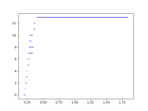
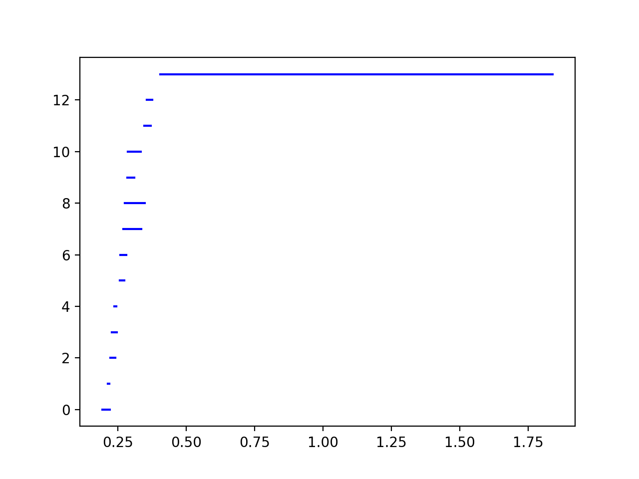
The 1-dimensional barcode, plotted below using the built-in Plotting functionality, reflects that we’ve sampled an annulus:

>>> d.plot.plot_bars(dgms[1], show = True)

(png, hires.png, pdf)

We select the longest bar and take its corresponding cocycle:

>>> pt = max(dgms[1], key = lambda pt: pt.death - pt.birth)
>>> print(pt)
(0.405474,1.83973)
>>> cocycle = p.cocycle(pt.data)

To smooth the cocycle and convert it to the corresponding circular coordinates, we need to choose a complex, in which we do the smoothing. Here we select the complex in the filtration that exists at the midvalue of the persistence bar, (pt.death + pt.birth)/2:

>>> f_restricted = d.Filtration([s for s in f if s.data <= (pt.death + pt.birth)/2])
>>> vertex_values = d.smooth(f_restricted, cocycle, prime)

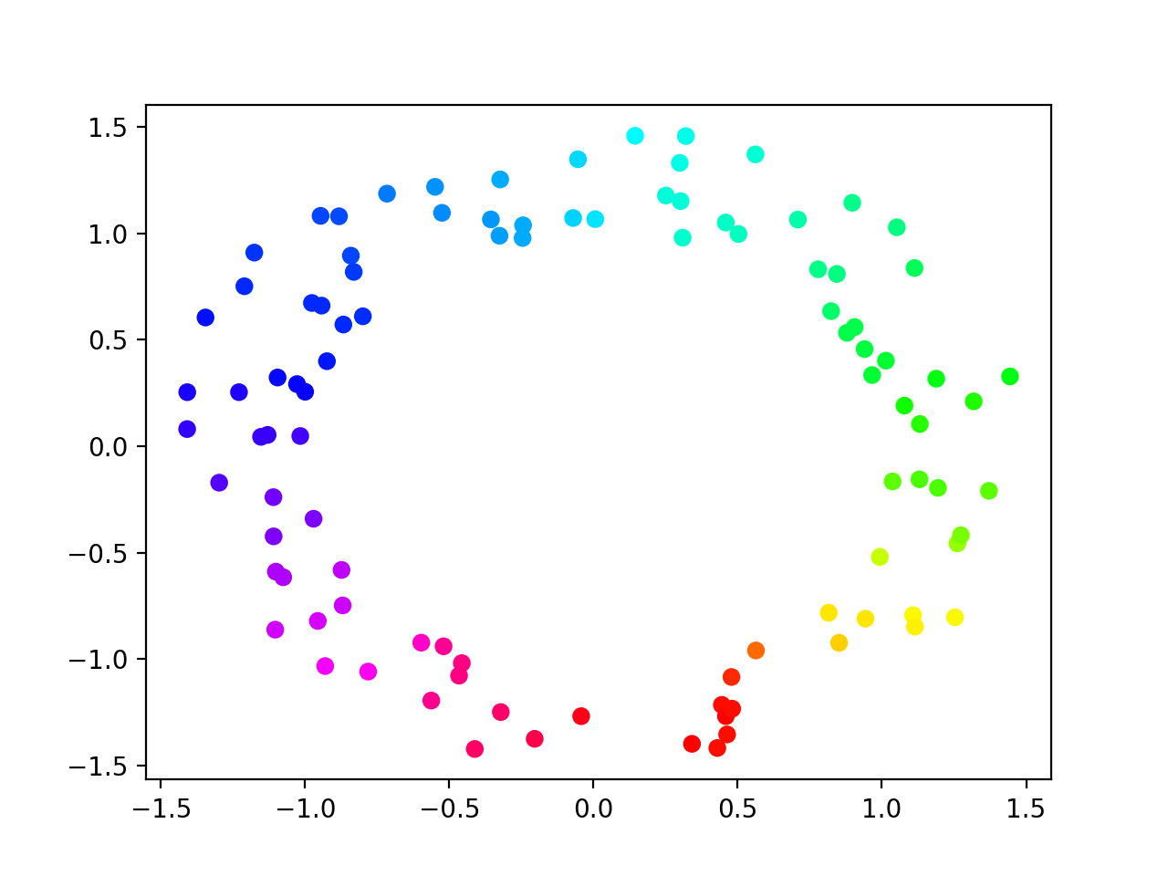
Now we can plot the points using hue to show the circular coordinate:

>>> import matplotlib.pyplot as plt
>>> plt.scatter(points[:,0], points[:,1], c = vertex_values, cmap = 'hsv')
<...>
>>> plt.show()

(png, hires.png, pdf)